Newsletter  2020.2  Index

Theme : "The Conference of Fluid Engineering Division (February issue)” Preface T. HASHIMOTO，S. MATSUDA，H.J. PARK Moving-boundary problems in rarefied gas dynamics Tetsuro TSUJI (Kyoto University) Flow Control of Jets and Separated Flows Toshihiko SHAKOUCHI (Mie University) Machine-learned three-dimensional super-resolution analysis of turbulent channel flow Kai FUKAMI, Koji FUKAGATA (Keio University), and Kunihiko TAIRA (UCLA) Flow control around an oscillating square cylinder by using plasma actuators Chihiro ONAHA (Toyohashi University of Technology) Dream to Sounds Takumi FUKUSHIMA (Tokyo University of science)

 

Machine-learned three-dimensional super-resolution analysis of turbulent channel flow

Kai FUKAMI Keio University	Koji FUKAGATA Keio University	Kunihiko TAIRA UCLA

Abstract

We present a machine-learning-based flow reconstruction method in space and time inspired by super-resolution analysis and inbetweening. The proposed model called a hybrid downsampled skip-connection multi-scale (DSC/MS) model based on convolutional neural network is utilized to reconstruct high-resolution flow field from grossly coarse low-resolution data in space and time. The present reconstruction procedure is illustrated with an example of two-dimensional decaying turbulence in Fig. 1. Spatial high-resolution data are obtained from low-resolution data, prepared by average sampling operation, using spatial super-resolution model Fx such that q(x_HR, t_LR) = F_x(q(x_LR, t_LR)). The flow fields that are spatially reconstructed at two instances t = nΔt and t = (n+k)Δt are then fed into model Ft for inbetweening (nonlinear temporal interpolation) to obtain flow fields at t = (n+1)Δt to t = (n+k-1)Δt. Through these procedures, we obtain high-resolution flow fields from low-resolution flow data formulated as

q(x_HR, t_HR) = F_t(F_x(q(x_LR, t_LR))).

As an example, we consider the turbulent channel flow at Re_τ = 180. The high-resolution field obtained by direct numerical simulation (DNS) has 128 × 48 × 128 grids in x, y, and z direction, respectively. As the counterpart, two coarseness are used: medium resolution (16 × 6 × 16 grids) and low resolution (8 × 3 × 8 grids). We present x-z sectional isosurfaces of the second invariant of the velocity gradient tensor (Q-value) of spatial super resolution reconstruction in Fig. 2. The vortex core structures do not appear with the low-resolution input at Q⁺ = 0.03 due to its extremely high coarseness. Note that we can see small structures with a lower threshold, e.g., Q⁺ = 0.005, as also shown in Fig. 2. With the use of the machine-learning-based super resolution, the reconstructed flow fields are in great agreement with the reference DNS data. The inbetweening reconstruction is then performed using the spatial reconstructed fields as summarized in Fig. 3. Here, we consider two ranges of time steps between the first and end snapshots: medium and wide time steps, respectively. The aforementioned time steps are set based on the temporal two-point correlation coefficients in the region near the wall. As the spatial input, the medium resolution which has 16 × 6 × 16 grids is applied. With the medium time step, the machine learning model can interpolate the flow field successfully in time. On the other hand, the vortex core structures are not reconstructed well with the wide time step, especially at t = (n+4)Δt because of the temporal coarseness. Summarizing above, the flow fields can be reproduced as long as the correlation is not too low.

Key words

Turbulence, Machine learning, Super resolution, Inbetweening

Figures

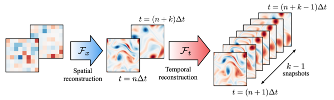
Fig 1.  Spatio-temporal super resolution reconstruction of two-dimensional turbulence.

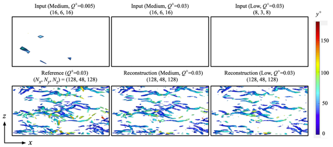
Fig 2.  Spatial super resolution reconstruction of turbulent channel flow.

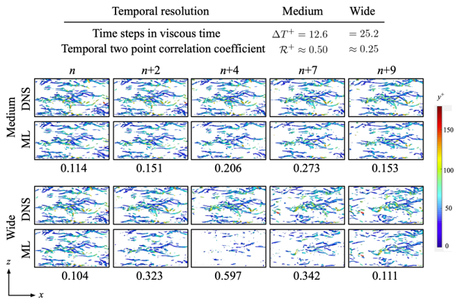
Fig 3.  Spatio-temporal super resolution reconstruction of turbulent channel flow. The listed values indicate the L₂ error.