

Newsletter 2022.11 Index
Theme : "Mechanical Engineering Congress, 2022 Japan (MECJ-22)”
|
Deep learning for viscoelastic fluids and turbulent diffusion
|

Abstract
In this study, we focus on the conformation stress field of viscoelastic turbulent channel flow (in §2), and passive-scalar turbulent diffusion in Newtonian turbulent channel flow (in §3). We aim to realize predictions by inferring those huge instantaneous turbulent-flow data, so-called “turbulence big data”, with aid of machine learning. More essentially, our attempt is to demonstrate feasibilities of predicting the physics inherent in turbulent phenomena or the external boundary conditions by machine learning.
Key words
Turbulence, Convolutional neural network, Surrogate model, Source estimation, Inverse problem
1. Introduction
In the literature, the physics in wall turbulence have been discussed with respect to those statistical features for the equilibrium state(1). The apparently random micro-scale turbulence (fluctuations) and eddies are often just averaged except for those that are of interest in the coherent structure related to the self-sustaining mechanism of wall turbulence. Although the understanding of the nature of wall turbulence and the prediction of the field have been based on statistical features, we would discuss the possibility of extracting significant features from the instantaneous field with the help of machine learning. Even the turbulent channel flow can be regarded as a non-equilibrium state in which turbulence generation, diffusion, and dissipation occur intermittently if viewed instantaneously and locally, and even apparently random turbulence and eddies may contain significant features that we might miss. If we can extract the unique features of instantaneous fields, which are lost by statistical processing, we expect to be able to predict the internal (intrinsic physics) and external (initial and boundary conditions) information from spatiotemporally limited information. Although there are various approaches to realize this, such as data assimilation and sparse sensing, the fact that direct numerical simulation (DNS) of the turbulent flows in addition to experiments inevitably accumulates instantaneous field data from moment to moment motivates us to utilize vast amounts of turbulence big data (Figure 1). In this study, we have investigated the possibilities of deep learning using convolutional neural networks (CNN), and here we report two test cases.
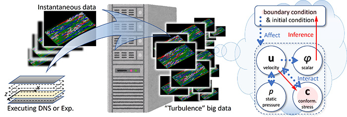
Figure 1 Inference of intrinsic physics and external conditions based on turbulence big data
2. Internal-physics prediction: Conformation stress field estimation for viscoelastic turbulence
In this section, we aim to deduce the conformation stress field of turbulent channel flow of a viscoelastic fluid, which is assumed to be a dilute surfactant or polymer solution that can reduce the turbulent frictional drag. This study also constructs a surrogate model to partially replace the highly loaded and numerically unstable DNS at high Reynolds numbers and high Weissenberg numbers. In general, constitutive equations such as the FENE-P model and the Giesekus model are used in numerical simulations of viscoelastic fluids, but numerical instability at high Weissenberg numbers is often problematic(2). We attempt to avoid this problem by conducting a data-based simulation instead of solving constitutive equation. In this study, DNS data based on the Giesekus model were trained by U-Net(3), a kind of CNN, to predict the instantaneous conformation stress field from the instantaneous velocity field at the same instance and location: see Figure 2. With using the trained U-Net, the feasibility of DNS-CNN integrated simulation (DNS only for velocity field calculation) was investigated.
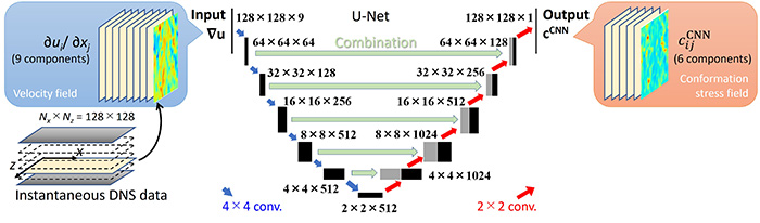
Figure 2 U-Net architecture and input and output data
Figure 3 compares the DNS (ground truth) and U-Net prediction results for a friction Reynolds number of 180 and a friction Weissenberg number of 10. Despite the use of a single learner, the characteristics of the viscous sublayer, buffer layer, and channel central layer were qualitatively well predicted. The correlation coefficients were also high, ranging from 0.7 to 0.9, but there is a tendency for the U-Net to underestimate strong local variations in the buffer layer. This may be due to the fact that strong near-wall coherent structures are dominant in the buffer layer, and those vortices do not necessarily exist in the reference plane (i.e., they are not included in the input information). Prediction accuracy tends to be similar for other stress components and at other Reynolds numbers (4).
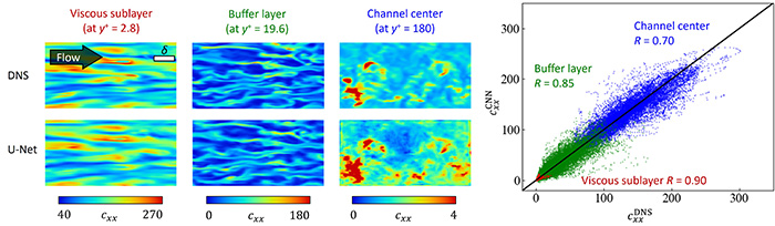
Figure 3 Predictions of instantaneous conformation stress fields from the turbulent velocity fields by U-Net, for a viscoelastic turbulent channel flow. (Left) Contours of the conformation stress in wall-parallel planes at different heights from the wall: y+ represents the wall-normal height in wall unit. Top and bottom rows are respectively the DNS and U-Net results at the same instance and locations. (Right) Scatterplot between the DNS and prediction values. The correlation coefficient is represented by R.
We have confirmed that the DNS-CNN integrated simulation runs stably and produces statistics close to the DNS (4), as shown in Movie 1. The RMSE (root-mean-square error) in the figure converges at around 1.0, which is comparable to the turbulent intensity and, thereby, such an error is not an essential issue, as it is due to the sensitivity to small differences, like a chaos. The aforementioned underestimation of local rare event in the buffer layer is not fatal to the surrogate-model simulation.
Movie 1 Reproduction of viscoelastic turbulent channel flow by DNS-CNN integrated simulation.
3. External-condition prediction: Estimation of scalar diffusion sources in turbulence
Solving inverse problems, such as immediately identifying the source of substance diffusion from limited instantaneous and localized concentration distribution information, is an important task in marine and chemical plants. An example of the former case is the search for hydrothermal deposits containing rare-metal resources, and in the latter case, the rapid response to hazardous substance leaks is needed. Many of these measurements should be made in turbulent environments, which increases the difficulty. As a solution to such technical requirements, we have applied deep learning, which can extract features from instantaneous two-dimensional information (images) and perform inference, to build a CNN learner that can estimate the diffusion source from downstream concentration information in turbulent scalar diffusion.
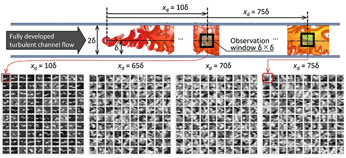
Figure 4 Problem setup of a scalar point source immersed in a turbulent channel flow and sample images obtained at several observation windows. (Top) The flow configuration and the point source. The distance from the point source is labelled as xd, which is the quantity estimated by the image recognition of CNN. (Bottom) Image samples for machine learning of scalar plume patterns, which were obtained by DNS.
The field of interest is a scalar diffusion from a stationary point source in a turbulent channel flow. As shown schematically in Figure 4, the distance xd to the diffusion source is deduced from the instantaneous concentration distribution (image) in a finite size observation window downstream of the point source. The task is to discriminate (classify or regression predict) multiple observation locations from the concentration distribution image.
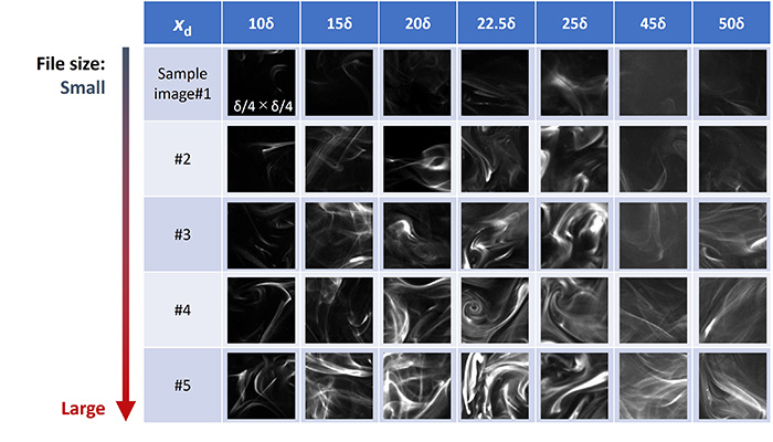
Figure 5 Image samples of dye plume pattern, used for validation of our pretrained CNN.
Training and validation images were prepared by experimentally-obtained PLIF (planar laser-induced fluorescence) images (5) or DNS data (6). Figure 5 shows typical snapshots by PLIF at each downstream locations, both of which were successfully recognized by our trained GoogLeNet (7) with a determination accuracy of over 80%.
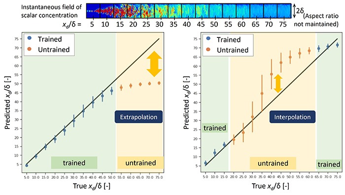
Figure 6 Estimation results of trained/untrained class. Left, the extrapolation; right, the interpolation.
The CNN trained on a set of images obtained from the DNS, as given in Figure 4, exhibited an estimation accuracy close to 100% when validated on data images not used for training. However, as shown in Figure 6, the accuracy significantly decreased when interpolated or extrapolated predictions of untrained classes were made (6). To improve this, it will be necessary to further identify the features that the learner extracts from instantaneous local information. For more details, please refer to our paper that discusses on CNN-architecture dependence, image-size dependence, and robustness to image rotation/scaling and noise (8).
4. Concluding remarks
Using deep learning, we demonstrated the estimation of the conformation stress field from the velocity field based on instantaneous local information, and the estimation of the diffusion point source location from the downstream concentration distribution. We demonstrated the usefulness of instantaneous local information, which is lost in statistics, and confirmed the possibility of using deep learning to construct a viscoelastic fluid surrogate model and a diffusion source estimation tool. The surrogate-model simulation using a learned CNN was confirmed to work and have the potential to avoid numerical instability. Many issues remain to be solved, including the handling of rare events, and the extrapolation as well as interpolation of untrained regions. In addition to improving learning accuracy, finding the learning limit will lead to clarification of intrinsic physics and data collection guidelines for external inference, so future research on machine learning of turbulence big data is highly anticipated.
In this research, we are using existing architectures. The above results may be further improved by the latest neural networks, but what is essentially important is not simply the improvement of estimation accuracy. In the case of the surrogate-model construction, inference that does not violate mathematical realizability and the physics laws should be guaranteed. In the case of image recognition, the identification of features is a crucial issue. For this purpose, PINN (Physics-Informed Neural Network) and GAN (Generative Adversarial Network) must be effective.
Acknowledgements
The authors would like to thank Mr. Takahiro Ishigami, Mr. Toshiyuki Kurihara, and Mr. Masaya Tashiro, graduate students at Tokyo University of Science, for their cooperation in this research. We used the supercomputer resources at the Cybermedia Center, Osaka University. This work was supported by JSPS Grants-in-Aid for Scientific Research (A) 18H03758 and (S) 21H05007, PI of which is Prof. Koji Fukagata (Keio University).
This article is a summary of my lecture given at the EFD Workshop held at the JSME Mechanical Engineering Congress in 2022. I would express my respect to the coordinators of the EFD Workshop over the years, especially to the organizers of this time:Prof. Shouichiro Iio (Shinshu University), Prof. Masaki Fuchiwaki (Kyushu Institute of Technology), Prof. Ayumi Inazawa (Tokyo Metropolitan University), and Prof. Satoshi Kikuchi (Gifu University). I would also like to thank Dr. Tetsuya Kanagawa (University of Tsukuba), Prof. Hideo Mori (Kyushu University), and the Publicity Committee of the Fluid Engineering Division, JSME, for giving me this precious opportunity to write this newsletter.
References