

Newsletter 2020.2 Index
Theme : "The Conference of Fluid Engineering Division (February issue)”
|
Moving-boundary problems in rarefied gas dynamics
Tetsuro TSUJI Kyoto University
|

Abstract
When a mean free path of gas molecules l is comparable to a characteristic length L of gas flows, the Knudsen number Kn = l/L, which indicates the degree of gas rarefaction, takes finite values. For such a situation, the framework of rarefied gas dynamics should be used to investigate the gas flows instead of ordinary fluid mechanics. This article describes some findings in a series of works by the author and a colleague on the numerical analysis of moving-boundary problems for the rarefied gases (Tsuji, T. & Aoki, K., J. Comput. Phys. 250, 574-600 (2013); Tsuji, T. & Aoki, K., Phys. Rev. E 89, 052129 1–14 (2014).). The moving-boundary problems of rarefied gases are found in engineering applications of vacuum technology and micro devices with moving parts. It has been clarified in the above references that the velocity distribution function of gas molecules has some singularities due to the unsteady motion of the boundary. These singularities are treated adequately in the numerical analysis by using the method of characteristics, and the velocity distribution functions are obtained precisely for the cases with intermediate Knudsen numbers, including the case of infinite Kn. The velocity distribution functions have discontinuities produced by the unsteady motion of the boundary, and they decay as time goes on due to the intermolecular collision. It should be remarked that a standard finite-difference scheme cannot reproduce the precise profile of the velocity distribution function. Furthermore, the decay of an oscillating plate due to the drag in a rarefied gas is numerically investigated, taking into account the above-mentioned singularities. The decay rate is found to be proportional to t-3/2 for large t and for an intermediate Kn, where t is a time variable. This rate of decay is different from that for Kn → ∞, indicating that the intermolecular collision affects the manner of decay.
Key words
Rarefied gas dynamics, Moving-boundary problems
Figures
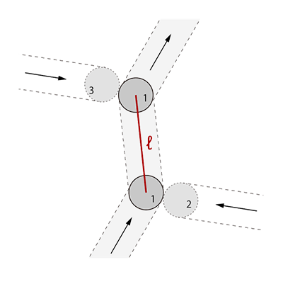
Figure 1 The definition of mean free path of gas molecules.
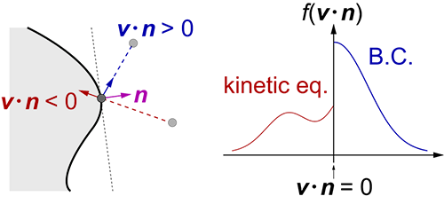
Figure 2 Gas molecules impinges on the boundary with a velocity v・n < 0 and are reflected with a velocity v・n > 0. The velocity distribution function on the boundary is discontinuous at v・n = 0. The discontinuity produced on the boundary can propagate into the gas domain along the characteristic curve.
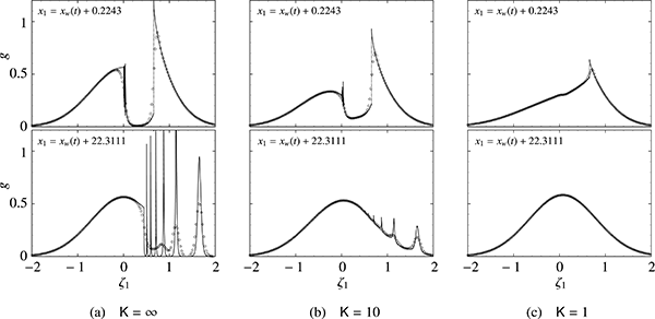
Figure 3 Velocity distribution functions of gas molecules in moving boundary problems. The boundary is an infinite plate oscillating in its perpendicular direction with the non-dimensional amplitude unity. g = g(x1, ζ1, t) is the non-dimensional marginal velocity distribution function, x1 and ζ1 are the non-dimensional position and molecular velocity in the direction of the oscillation of the plate, respectively, xw(t) is the non-dimensional position of the plate, and K is the parameter of the order of Knudsen number. Solid lines are obtained using the method of characteristics, while symbols are obtained by a standard finite-difference scheme. The former captures the details of the velocity distribution function including discontinuities but the latter fails. This figure is reprented from Ref. (1) under the permission of Elsevier.
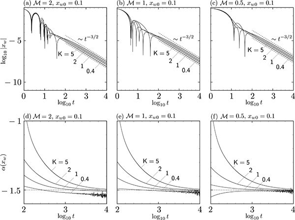
Figure 4 log10|xw| versus log10 t for long times at several K for xw0 = 0.1, vw0 = 0. (a) M = 2, (b) M = 1, and (c) M = 0.5. Panels (d), (e), and (f) show, respectively, the gradient of the curves in panels (a), (b), and (c). This figure is reprented from Ref. (2) under the permission of American Physical Society.